Bundled examples

The examples/ directory contains runnable scripts demonstrating the package’s core workflows. Every example accepts --help for a full list of options and --list-interfaces for a table of all bundled interfaces.

Quick reference

Script	What it demonstrates	Default interface	Runtime
bilayer_relaxation.py	Two-layer moire relaxation	Graphene/Graphene (0.2 deg)	2-3 min
multilayer_penetration.py	Relaxation penetration through a multi-layer stack	Graphene/Graphene (0.035 deg, 60/60)	10-30 min
strain_extraction_and_pinning.py	Inverse strain extraction + constrained relaxation	MoSe2/WSe2 H	seconds
spatial_strain_relaxation.py	End-to-end strain extraction from data + relaxation	MoSe2/WSe2 H	~10 min
tdbg_low_twist_relaxation.py	TDBG 2DW network at very low twist	TDBG-DFTD2 (0.02 deg)	~7-8 min

bilayer_relaxation.py

The main bilayer relaxation script. Runs any two-layer moire system (homobilayer or heterointerface) and produces stacking energy, elastic energy, and local twist angle maps.

Presets

Three named presets reproduce the classic demonstrations:

# Twisted bilayer graphene (default)
python bilayer_relaxation.py

# Graphene on hBN (pure lattice-mismatch moire)
python bilayer_relaxation.py --preset hbn

# H-stacked MoSe2/WSe2 (deep moire potential)
python bilayer_relaxation.py --preset tmd

Preset	Interface	Twist	Pixel size	Method	Max iter	gtol
graphene	graphene	0.2 deg	1.0 nm	newton	60	1e-6
hbn	graphene-hbn	0.0 deg	0.5 nm	L-BFGS-B	300	1e-4
tmd	mose2-wse2-h	1.5 deg	0.5 nm	L-BFGS-B	300	1e-4

Any explicit CLI flag overrides the preset value:

python bilayer_relaxation.py --preset tmd --theta-twist 3.0

Sample output: twisted bilayer graphene (0.2 deg)

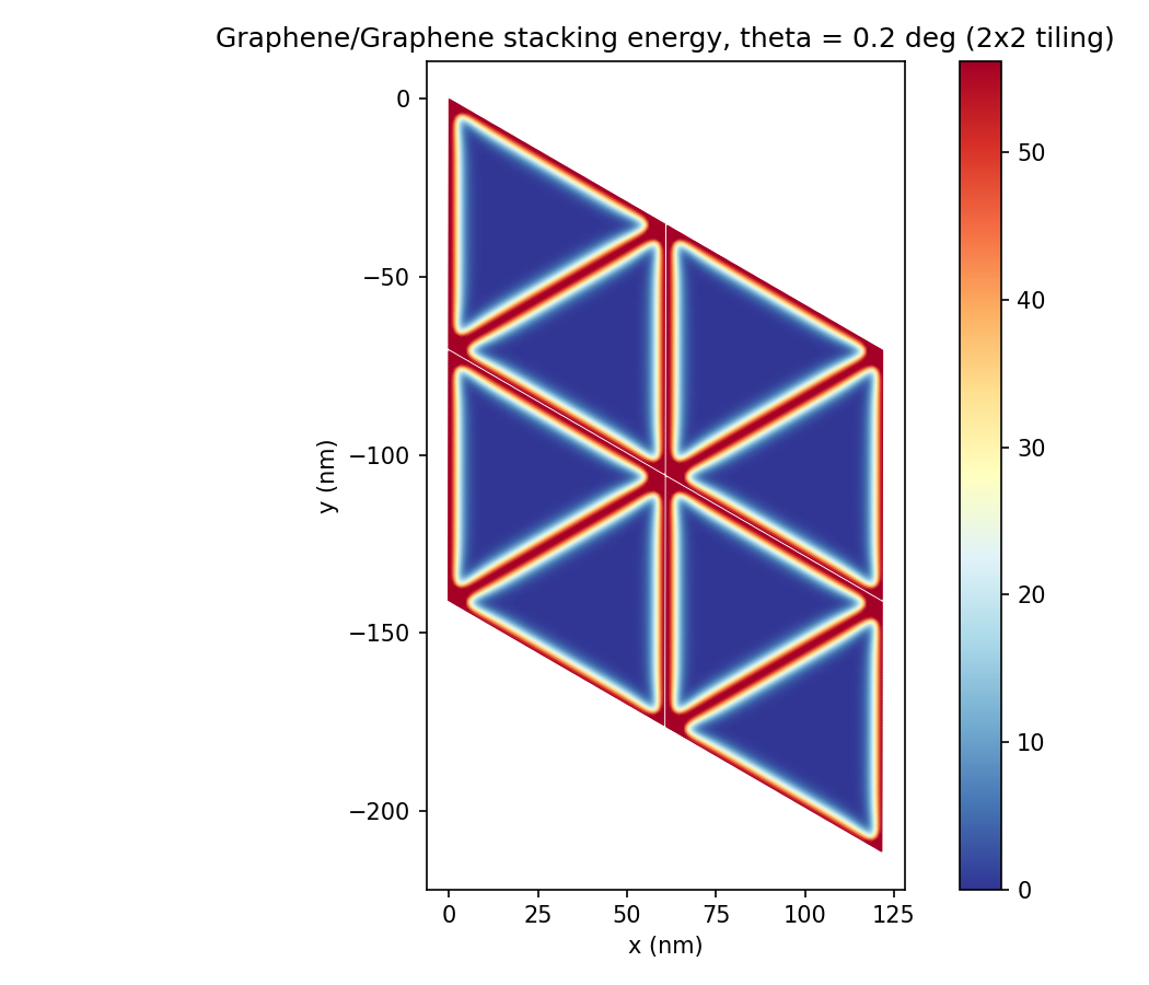
Stacking energy density showing the hallmark AB/BA triangular domain pattern with narrow domain walls (soliton network).

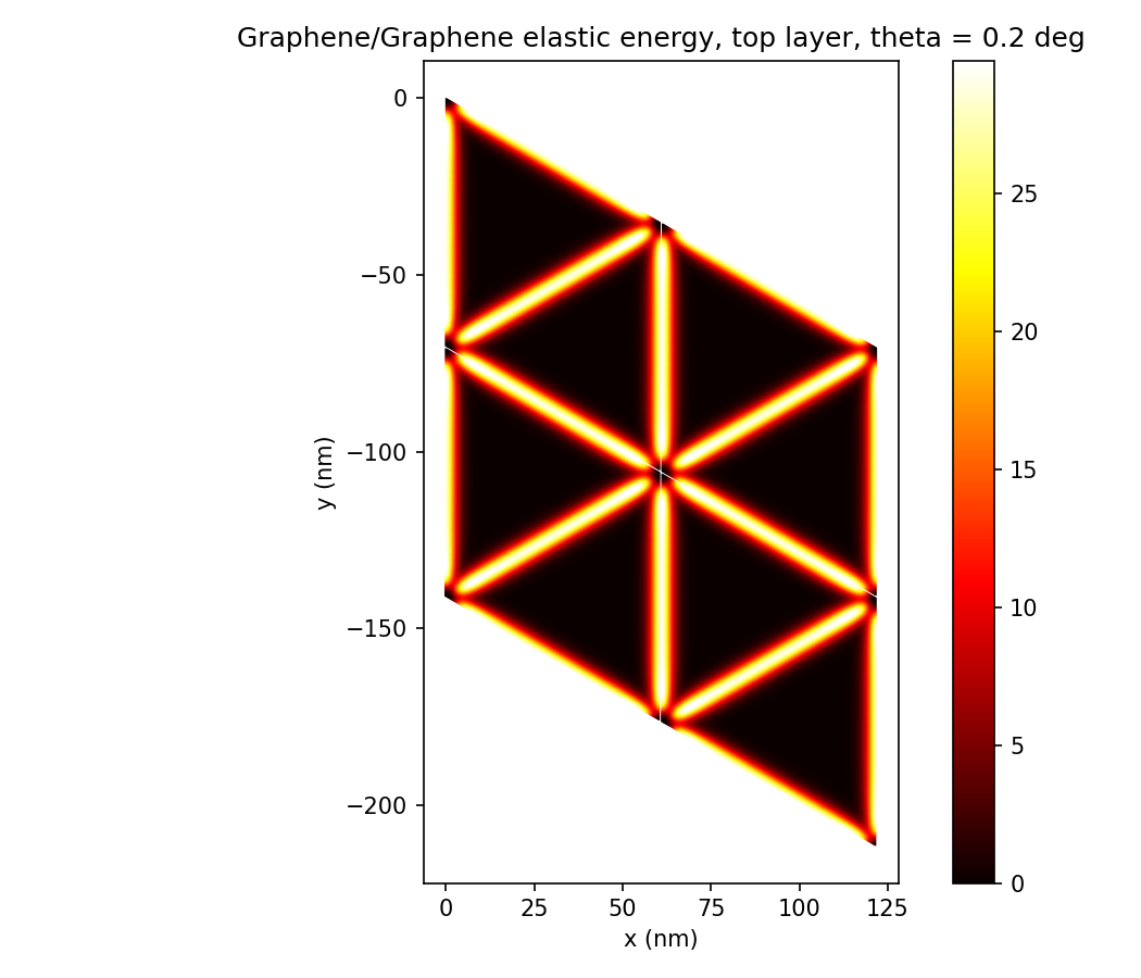
Elastic energy density concentrated along the domain walls, forming the strain-driven soliton network.

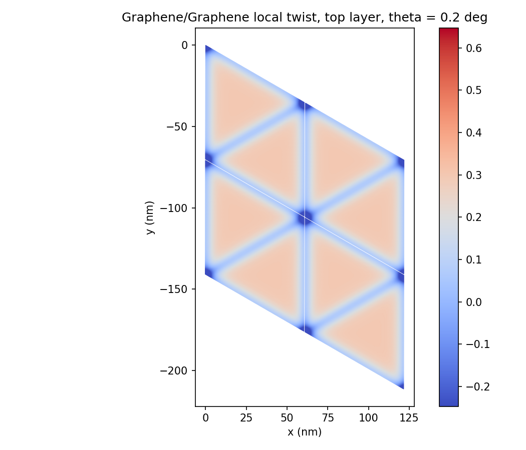
Local twist angle map showing enhanced twist at AA vortex sites and reduced twist in the relaxed AB/BA domains.

Sample output: graphene/hBN (0 deg, lattice-mismatch moire)

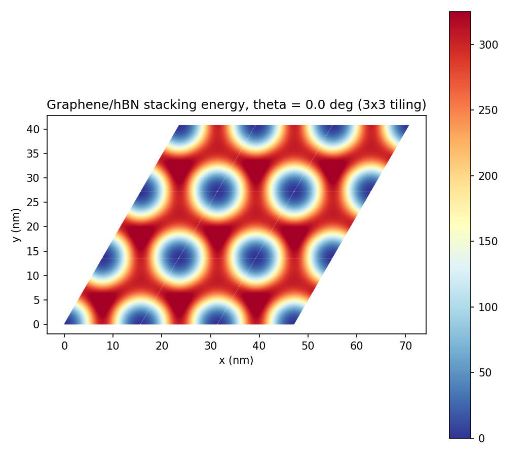
Graphene on hBN at zero twist. The 1.6% lattice mismatch drives a moire pattern with a single energy minimum per cell.

Sample output: MoSe2/WSe2 H-stacked (1.5 deg)

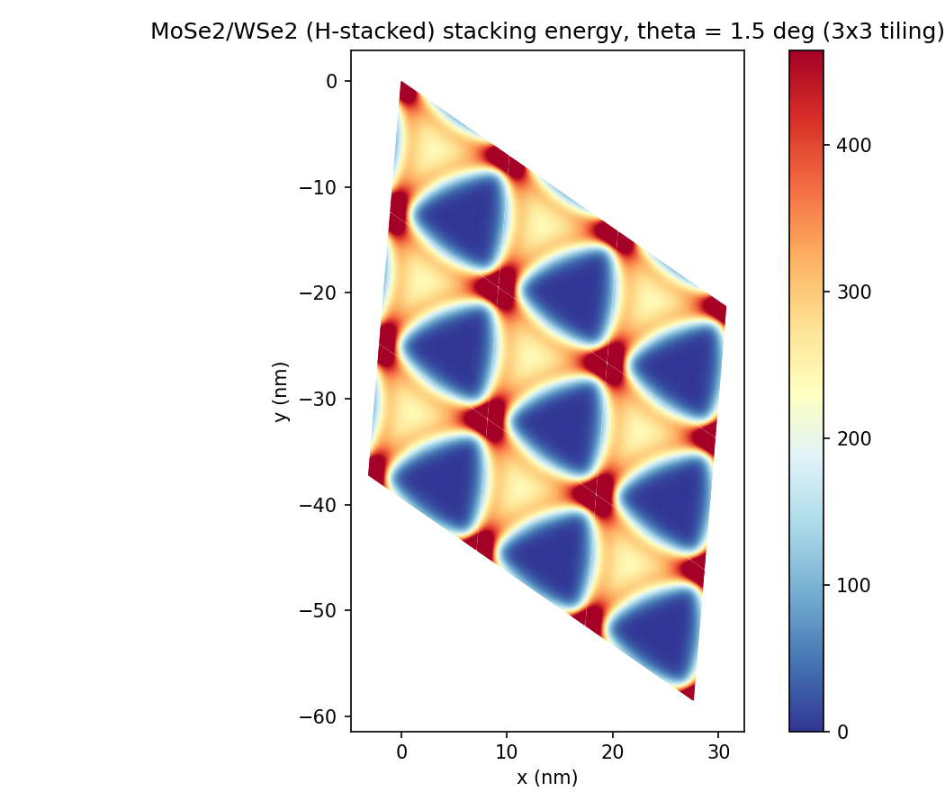
H-stacked MoSe2/WSe2 stacking energy. The broken inversion symmetry produces three distinct stacking minima (XX’, MX’, MM’) per moire cell, unlike the two-fold AB/BA pattern of graphene.

Custom interface from TOML

python bilayer_relaxation.py --interface my_interface.toml --theta-twist 0.5

See custom-materials.md for the TOML schema.

Key CLI arguments

Flag	Description	Default
--interface	Bundled name or TOML file path	graphene
--preset	Named preset (graphene, hbn, tmd)	graphene
--theta-twist	Twist angle in degrees	0.2
--pixel-size	Mesh element size in nm	1.0
--method	Solver: newton, L-BFGS-B, pseudo_dynamics	newton
--max-iter	Max solver iterations	60
--gtol	Gradient tolerance	1e-6
--force	Re-solve, ignoring cache
--no-plots	Skip plot generation
--output-dir	Output directory	examples/output/
--list-interfaces	Print all bundled interfaces and exit

Outputs

All outputs are named by a slug derived from the interface name (e.g. graphene_graphene_stacking.png):

• <slug>_relaxed.npz – cached relaxed state

• <slug>_stacking.png – GSFE / stacking energy density

• <slug>_elastic.png – elastic energy density (top layer)

• <slug>_twist.png – local twist angle map

• <slug>_summary.txt – scalar diagnostics

multilayer_penetration.py

Demonstrates how moire relaxation penetrates deep into a multi-layer substrate. Only homobilayer interfaces are supported (the internal flake stacking requires the same material on both sides).

# Default: 60/60 graphene at 0.035 deg
python multilayer_penetration.py

# Smaller stack, faster
python multilayer_penetration.py --n-top 5 --n-bottom 12 --theta-twist 0.5

# hBN homobilayer
python multilayer_penetration.py --interface hbn-aa --theta-twist 0.5 --n-top 5 --n-bottom 12

Additional flags: --n-top, --n-bottom, --min-mesh-points, --linear-solver, --linear-solver-tol, --linear-solver-maxiter.

If you pass a heterointerface or a TOML-loaded interface without a stacking function, the script exits with a clear error message.

Sample output: 60/60 graphene at 0.035 deg

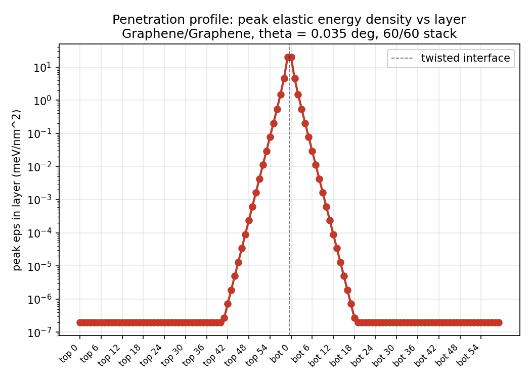
Peak elastic energy density vs layer index. Relaxation decays exponentially from the twisted interface into both flakes.

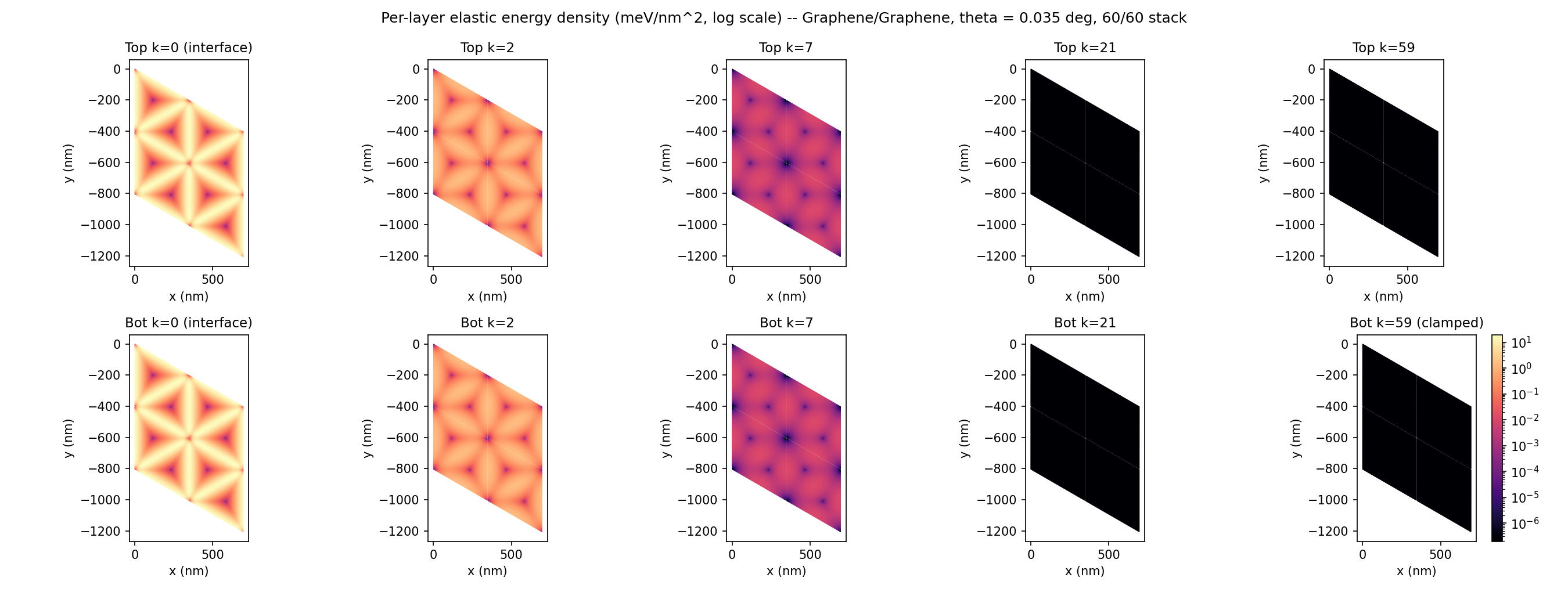
Per-layer elastic energy density maps showing the soliton network fading as it penetrates deeper into the stack.

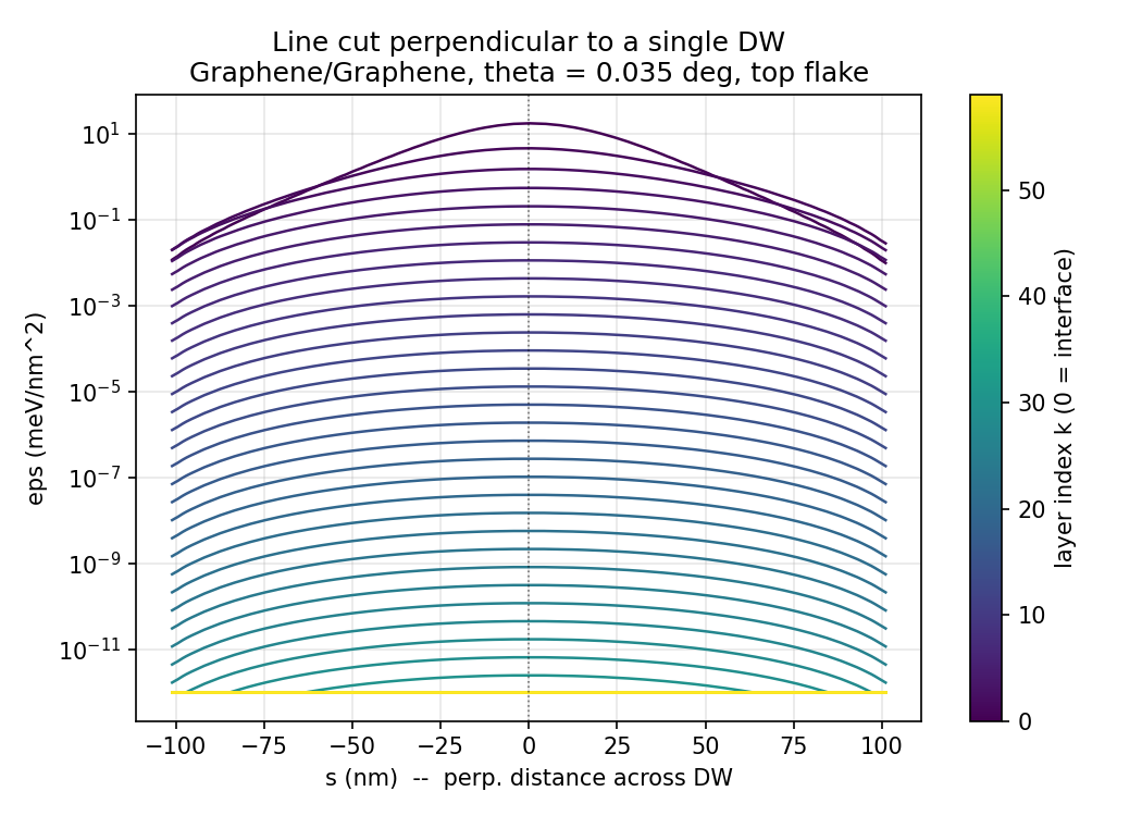
Domain-wall line cuts showing broadening of the soliton network with increasing depth from the twisted interface.

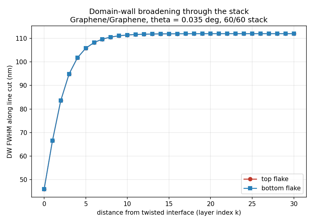
Domain-wall FWHM vs layer index, quantifying the broadening.

strain_extraction_and_pinning.py

Two-part example:

• Part A: Inverse strain extraction sweep (no relaxation). Recovers twist angle and strain from moire lattice vectors, sweeping the inter-vector angle.

• Part B: Constrained finite-mesh relaxation with imposed heterostrain. Pins high-symmetry sublattice sites to a uniform strain field and relaxes the GSFE + elastic energy.

# Both parts with defaults
python strain_extraction_and_pinning.py

# Only Part B with a different interface
python strain_extraction_and_pinning.py --skip-part-a --interface graphene-hbn --theta-twist 0.3

# Custom heterostrain
python strain_extraction_and_pinning.py --heterostrain 0.02

Sample output: Part A strain extraction sweep

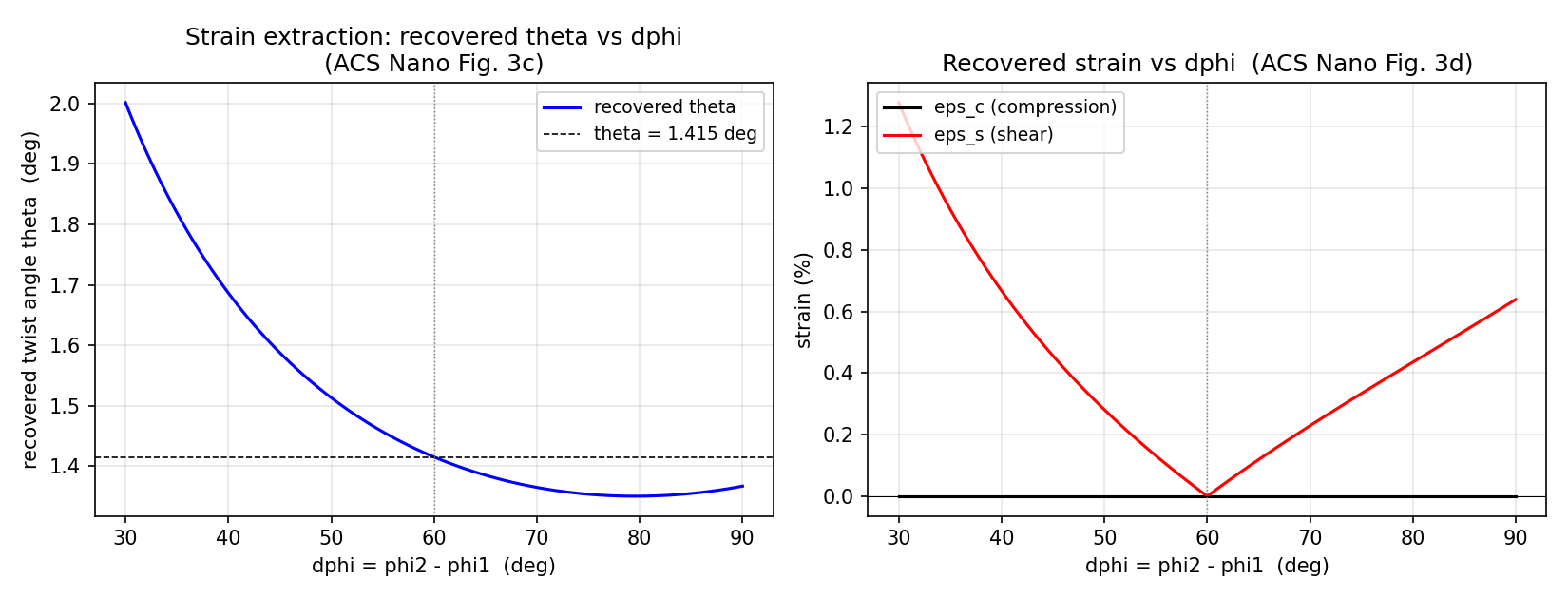
Recovered twist angle (left) and strain components (right) as a function of the inter-vector angle, reproducing Fig. 3c-d of Halbertal et al., ACS Nano 16, 1471 (2022).

spatial_strain_relaxation.py

End-to-end pipeline: loads polyline data from a CSV file, fits registry polynomials, extracts the spatially-varying strain field, and runs a constrained relaxation. Reproduces Fig. 1c-e of Halbertal et al. ACS Nano 16, 1471 (2022).

The bundled polyline data is at examples/data/mose2_wse2_polylines.csv. All pipeline parameters are configurable:

python spatial_strain_relaxation.py --poly-degree 11 --phi0 -65.6 --n-cells 55

Sample output

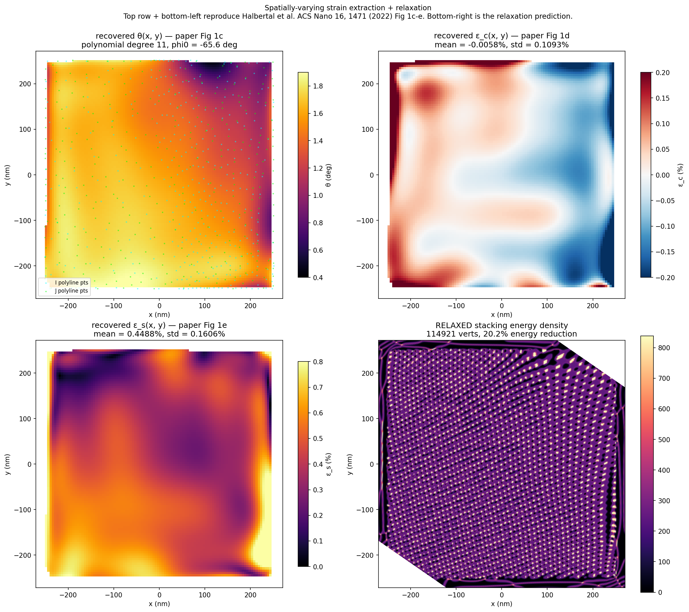
Four-panel headline figure. Top row + bottom-left reproduce the spatially-varying strain extraction from traced moire fringes (twist angle, compression strain, shear strain — cf. paper Fig. 1c-e). Bottom-right shows the constrained relaxation result: the equilibrium stacking-energy density aligned with the traced polylines.